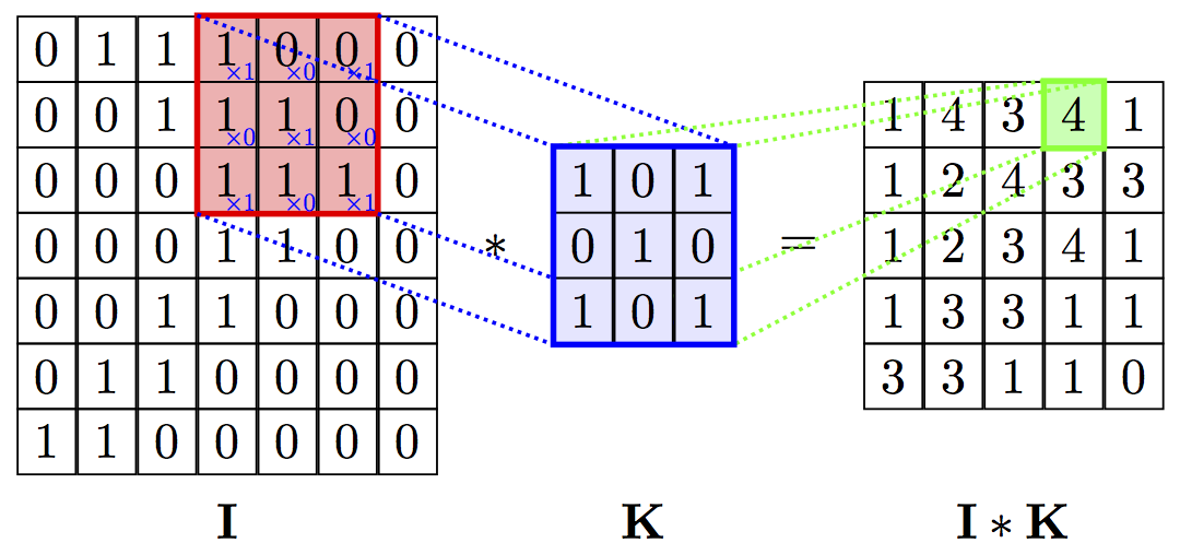
Fig. 1: Visual illustration of 2D convolution [2]
Filters, also known as kernels or masks, operate in the neighborhood of a pixel by applying a certain function to the neighbor pixels of the corresponding input pixel [1]. The neighborhood of a pixel contains a set of pixels that are closest to the pixel in the spatial domain, and the size of the set is determined by the kernel size.
Linear filters define the value of an output pixel as a linear combination of the values of neighbor pixels. The operation to apply these filters to an image is called convolution. 2D convolution in the spatial domain is defined by a matrix of weights, known as filters or kernels, where each weight is multiplied with the corresponding neighbor pixel of an input pixel and summed together to obtain the corresponding output pixel.
Fig. 1: Visual illustration of 2D convolution [2]
Some well-known linear image filters are smoothing filters, such as mean filters, which take the average of neighbor pixels, Gaussian filters, an approximation of Gaussian function, and sharpening filters for edge enhancement, such as Laplacian filter, a second order derivative mask, or linear unsharp masks, which highlight the high frequency components by first extracting, then adding them to the original image.
Although these filters perform well in many tasks, such as eliminating random noise, or extracting edges from an image, their expressive power is limited by their linear structure.
Nonlinear filters have the advantage of higher expressive power; hence, they allow us to implement advanced and novel image enhancement and manipulation techniques [3]. Such filters take image structure, such as edges, into account and apply spatially-varying functions to local image regions to preserve edges. This approach comes from the observation that image contents and complex manipulations are more likely to be piecewise smooth instead of being solely band-limited. Fig. 2 shows a 1D example of such piecewise smooth signals along with an example of domain transform application for edge-preserving filtering.
![]()
Fig. 2: 1D edge-preserving filtering using a piecewise linear function ct(u). (a) Input signal I. (b) ct(u). (c) Signal I plotted in the transformed domain (Ωw). Signal I filtered in Ωw with a 1D Gaussian (d) and plotted in Ω (e) [4].
Unlike spatially-invariant filters, edge-preserving filters can treat local image regions differently to preserve edges and apply more sophisticated manipulation techniques. However, this advanced approach comes at a price: computational complexity. Recently, methods to reduce the complexity of such algorithms have been discussed, which I will briefly mention in the following sections while discussing some common edge-preserving filters, namely bilateral filters and local laplacian filters.
A bilateral filter is a nonlinear operator that smoothes an image while retaining its strong edges. The success of the bilateral filter in edge preservation comes from the fact that it reduces the weights of nearby pixels whose values largely differ from the input pixel.
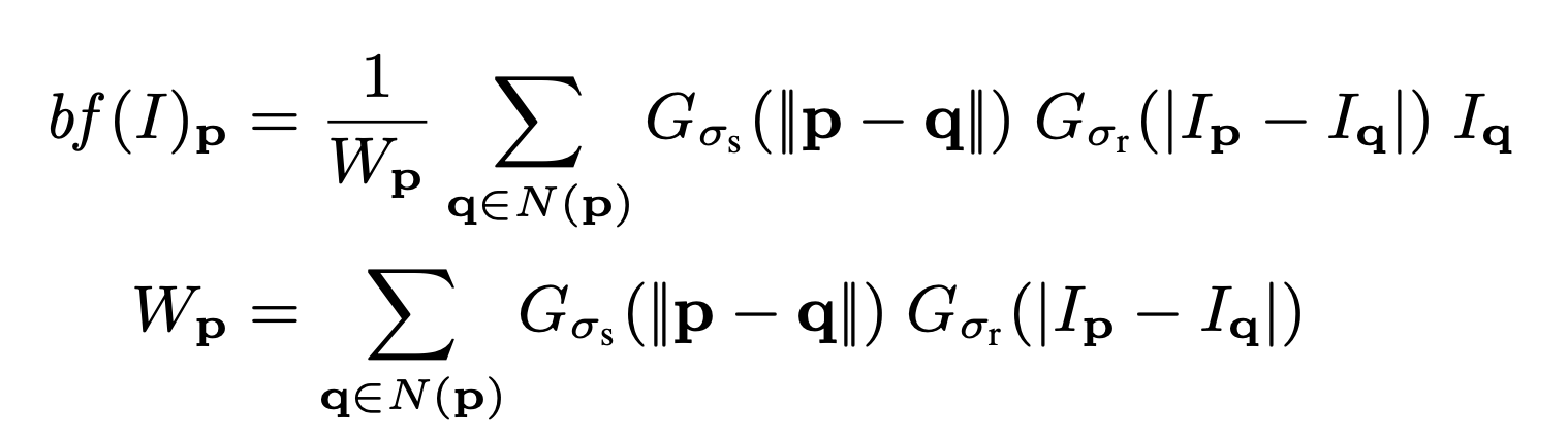
Eqn. 1: Bilateral filter definition for an image I, at position p [5]
Here, Gσs is a Gaussian on the spatial distance and Gσr a Gaussian on the pixel value difference. The output pixel is a weighted average where the weight is the product of Gσs and Gσr, the latter, also known as the range weight, disentangling pixels on one side of a strong edge from those on the other side so that the range variation in pixel values wouldn’t smooth strong edges [3].
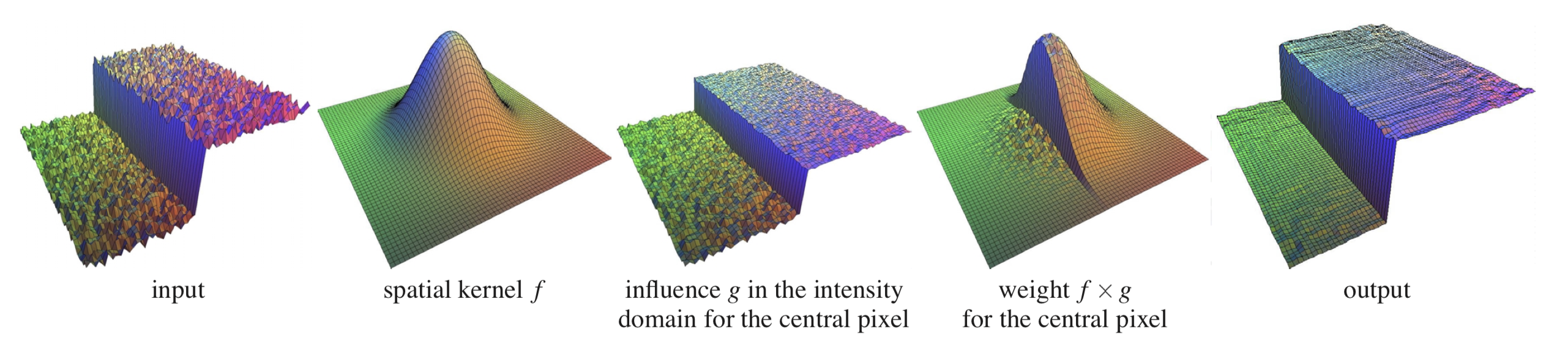
Fig 3. Bilateral filtering. The spatial and range kernels, f and g respectively, combine to preserve edges [6].
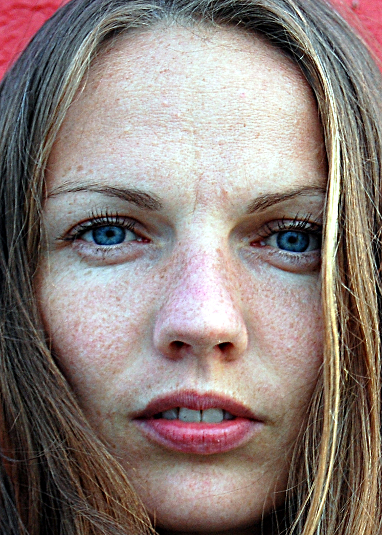

Fig 4. Illustration of bilateral filtering. Left: original image, right: bilateral-filtered image
The computational complexity of a direct implementation of bilateral filtering would be O(r2) per pixel, where r is the kernel radius. Later, different methods to reduce this complexity have been developed, among which the leading algorithm has a complexity of constant-time O(1) per pixel. Even with constant time per-pixel complexity, the overall complexity of bilateral filtering would become O(n2) time, where n is the number of pixels in an image. Since bilateral filtering is a spatially-varying function due to the range weight, a convolution, which can be highly accelerated with Fast Fourier Transform, cannot be directly applied to reduce the overall complexity. Therefore, alternative methods, such as a piecewise-linear approximation of a bilateral filter in the intensity domain and sub-sampling in the spatial domain [6], or redefining the algorithm as a higher dimensional convolution followed by trilinear interpolation and a division [7], or constructing a 3D array data structure, a bilateral grid [3], that combines the 2D spatial dimension with 1D range dimension, have been developed.
Local Laplacian filters are another type of edge-preserving filters where Laplacian pyramids are utilized. Laplacian pyramids have been long neglected for edge-preserving filtering due to the isotropic, spatially-invariant and smooth Gaussian filters on which pyramids are constructed [8]. However, a local laplacian filter benefits from local processing in which it modifies each coefficient of the pyramid levels separately which better allows the filter to distinguish edges from details.
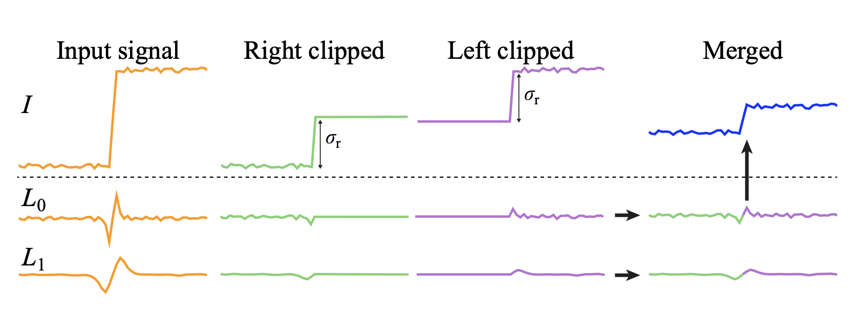
Fig 5. 1D local laplacian filter implementation. L0 and L1 represent the first two laplacian levels [8].
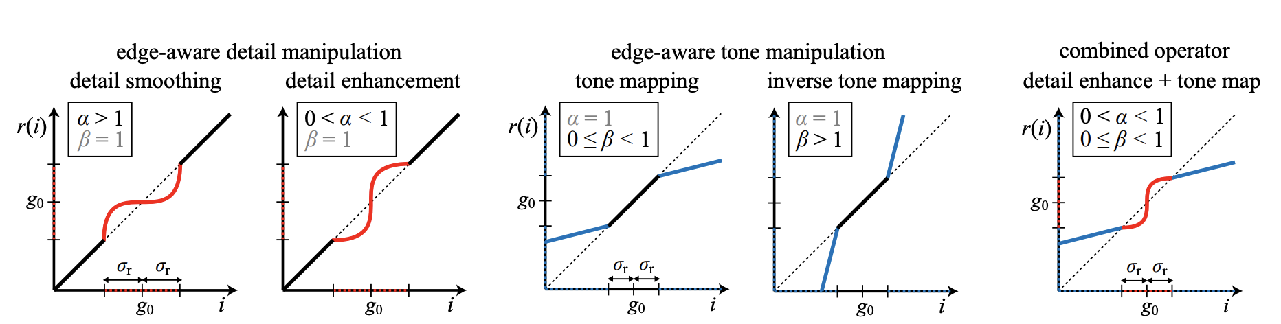
Fig 6. A variety of pointwise functions r(i) applied to a local value go to obtain the intermediate image [8].
A local laplacian filter renders an intermediate signal I’ for each pyramid coefficient (xo , lo), which is defined by the location and the pyramid level, based on the local signal value. First, values of the original signal are compressed into the range between (local value - σr) and (local value + σr) and the intermediate signal is rendered. Later, its Laplacian pyramid is built and its values are copied to the output pyramid. The threshold σr helps distinguish intricate details (red curve) from strong edges (blue curve).


Fig 7. Local laplacian filtering. Left: original image, middle: filtered image with parameters α=0.7 and β=0.4, right: filtered image with parameters α=2 and β=0.2
[1] MathWorks-Image filtering
[2] https://petar-v.com/GAT/
[3] Real-time edge-aware image processing with the bilateral grid
[4] Domain Transform for Edge-Aware Image and Video Processing
[5] Real-time Edge-Aware Image Processing with the Bilateral Grid
[6] Fast bilateral filtering for the display of high-dynamic-range images
[7] A fast approximation of the bilateral filter using a signal processing approach
[8] Local Laplacian Filters: Edge-aware Image Processing with a Laplacian Pyramid